Introduction: a variational DL solver based on DD method -> Deep DDM
benefits: complexity and generalization, mesh-free and data-free, parallel
Solution Method
variational principle 用变分法解?
\[\min E(u) = \int_\Omega \frac12 |\nabla u|^2 dxdy - \int_\Omega f \cdot u dxdy \\ \text{s.t. } u = 0 \text{ on } \partial \Omega\]Lagrangian problem: use lagrange multiplier $q$:
\[L(u, q) = \int_\Omega \frac12 |\nabla u|^2 dxdy - \int_\Omega u \cdot f dxdy + q \int_{\partial \Omega } u^{\2} dxdy\]Define flux $\tau$ in H(div) which is a symmtric tensor field in $H^1$ space, in which functions and divergence are both in $L^2$. Then we obtain
\[\begin{cases} \tau = - \nabla u, & \text{in } \Omega\\ \nabla \cdot \tau = f, &\text{in } \Omega \end{cases}\]The mixed residual loss
\[L(\tau,u ,q) = \int_\Omega [(\tau + \nabla u)^2 + (\nabla\cdot \tau - f)^2 ] dxdy + q\int_{\partial \Omega} u^2 dxdy\]Variational Priciple -> NN
$N_u(x,y;\theta_u), N_\tau(x,y;\theta_\tau)$: parameter -> approximate the solution at $(x,y) \in \Omega$. Loss function:
\[\min_\theta \int_\Omega [(N_\tau + \nabla N_u)^2 + (\nabla \cdot N_\tau - f)^2 ] dxdy + q\int_{\partial \Omega} N_u^2 dxdy\]We pick randomly a batch of m points in $\Omega$ and $n$ points on $\partial \Omega$ , and update perameters as:
\[\theta^{(k+1)} = \theta^{(k)} - \nabla_\theta \frac1m \sum_{i=1}^m [\cdots] - \nabla_\theta \frac1n \sum_{j=1}^n [\cdots]\]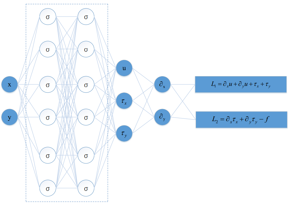
- tanh activation function
- PyTorch auto differentiation
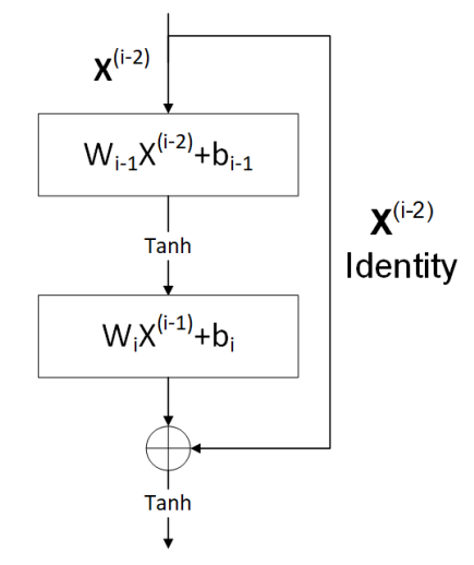
- Residual Network
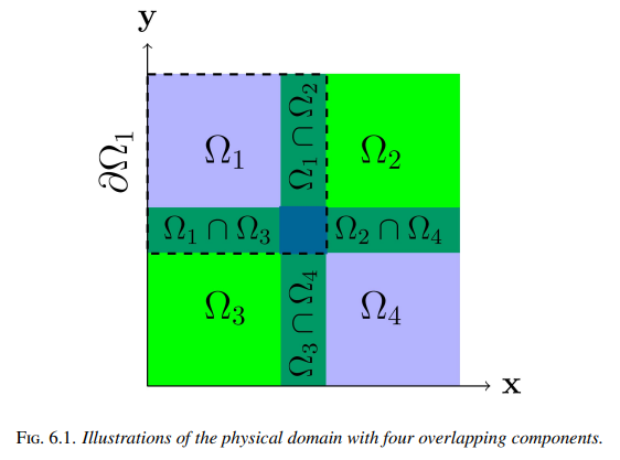
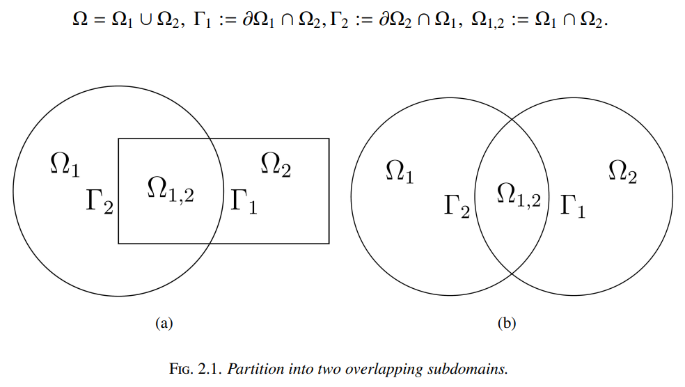
D3M
improve Schwarz alternating method with a better inhomogeneous D3M sampling method at junctions $\Gamma_i$ to accelerate convergence
Def. (Boundary function) A smmoth function $g(x,y)$ is called a boundary function associated with $\Omega$ if:
\[g(x,y) = \exp[-a \cdot d((x,y), \partial \Omega)] u(x,y)\]with $a» 1$. we have $g(x,y) = u(x,y)$ on boundary, and it decreases sharply as $d$ increases. Define v = u-g, we have
\[-\nabla^2 v = f + \nabla^2 g \text{ in } \Omega,\\ v = 0 \text{ on } \partial \Omega,\\ \tau = -\nabla v_i \text{ in } \Omega_i,\\ \nabla \cdot \tau = f + \nabla^2 g_i \in \Omega_i\]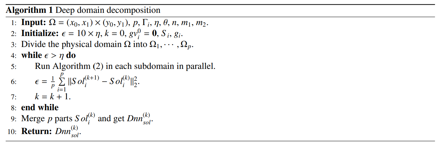
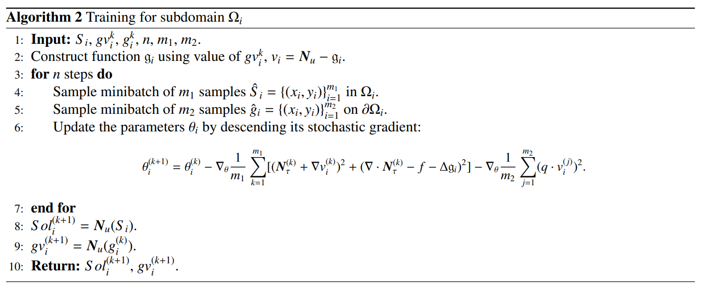
Solving Pipeline
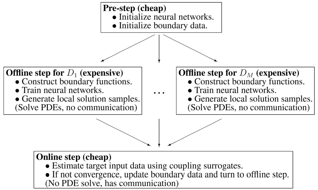
Analysis
Numerical Test
Poisson’s Equation
\[\begin{cases} - \nabla^2 u(x,y) = 1, &\text{ in } \Omega = (-1,1)\times (-1,1)\\ u(x,y) = 0, &\text{ on } \partial \Omega \end{cases}\]- randomly sample in each subdomain, and the number of samples increases with iteration times increase.
- The sample size on interfaces remains the same to provide an accurate solution for data exchange.